L17 GreyAtmosphere (template)

We start by importing the modules

• Numpy – operations on arrays and matrixes (and pi)

• Matplotlib pyplot – plotting library

• Matplotlin patches – module that enables patches in plots

• Astropy units – defined quantities with units. We also import the CDS conversions

• Scipy special – enable the use of the exponential integral function

• Astropy convolution – we will use this to smooth the spectrum of the sun

import numpy as np, copy
import matplotlib.pyplot as plt
%matplotlib inline
from astropy import constants as const
import astropy.units as u
from astropy.units import cds
cds.enable() 

from scipy.special import expn
from astropy.convolution import convolve, Box1DKernel

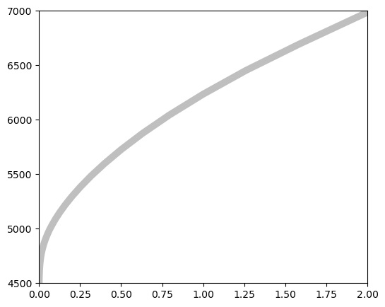
1. In class: Temperature structure of the Sun

Here, I provide a file containing (among other things) the temperature structure of the atmosphere of the sun resulting from a detailed model of the Sun’s atmosphere (numerical solution involving all 9 equations).

We will compare this to the analytical estimate we obtained by making the approximation that the opacity (\(\kappa\)) is “grey” (not dependent on wavelength). We also had to use one equation resulting from making a further approximation that the optical depth (\(\tau\)) is large.

So let’s see how good/bad this approximation actually is!

TODO: In the text below, please write down the equation you are using for \(T(\tau)\) in latex format.

TODO: In the graph below, add a curve that shows the approximation for \(T(\tau)\) assuming that the correction factor \(q(\tau)=0.7104 - 0.133\mathrm{e}^{-3.4488\tau_z}\).

TODO: In the graph below, add a curve that shows the approximation for \(T(\tau)\) assuming that the correction factor \(q(\tau)\sim \frac{2}{3}.\)

TODO: don’t forget to add axis labels and a legend to your graph.

file_url = "https://raw.githubusercontent.com/veropetit/PHYS633-F2024/main/Book/L17-GreyAtmosphere/17-sun_model.txt"
data = np.genfromtxt(file_url, skip_header=24, skip_footer=229, usecols=(1,2,4), names=True)

fig, ax = plt.subplots(1,1, figsize=(6,5))
ax.set_xlim(0,2)
ax.set_ylim(4500,7000)

ax.plot(10**data['lgTauR'], data['T'], label='Sun', lw=7, c="0.75")


# Define the effective temperature used for the solar model
Teff = 5777.0
#---------------------------------------
# In class




#------------------------

TODO: Please write a small paragraph with an interpretation of the result obtained:

2. Provided function: Calculation of the \(C(\alpha, \tau)\) function

In the worksheet in classe you derived this expression for the specific flux in a layer of depth \(\tau\) in a grey atmophere:

\[F_\alpha(\tau) = \frac{4\pi k^4T_\mathrm{eff}^4}{c^2 h^3} \alpha^3 \left[ \int_{\tau'=\tau}^\infty \frac{E_2(t-\tau)d\tau'}{e^{\alpha p(\tau')}-1} - \int_{\tau'=0}^\tau \frac{E_2(\tau-\tau')d\tau'}{e^{\alpha p(\tau')}-1} \right],\]

where the term in brackets is \(C(\alpha, \tau)\), and \(\alpha=hc/\lambda kT_\mathrm{eff}\) and \(p(\tau)=T_\mathrm{eff}/T(\tau)\).

The function below accepts a single value of \(\alpha\) and a single value of \(\tau\). It returns the value of \(C(\alpha, \tau)\) (The quantity in brackets).

def p_function(tau):
    
    q = 0.7104 - 0.133*np.exp(-1*3.4488*tau)
    p = 1.0 / ( 0.75 * (tau + q))**0.25
    return(p)

def c_function(alpha, tau):
    
    # create values of t for the integration
    tau_prime_low = np.linspace(0,tau, 1000)
    tau_prime_high = np.linspace(tau, 20, 1000)
    
    # Do the first integral
    y = expn(2, tau_prime_high - tau) / ( np.exp( p_function(tau_prime_high) * alpha)-1 )

    int_high = np.trapz( y, tau_prime_high)
    
    y = expn(2, tau - tau_prime_low) / (np.exp( p_function(tau_prime_low) * alpha)-1 )
    int_low = np.trapz( y, tau_prime_low)
    
    C = int_high - int_low
    
    return(C)

3. Let’s make a graph of the specific flux for various layers in the atmosphere.

In the class worksheet, we found that \(F_\alpha / \tilde{F}\) can be expressed as

\[ \frac{F_\alpha(\tau)}{\tilde{F}} = \frac{30}{\pi^4} \alpha^3 C(\alpha, \tau).\]

TODO:

Use the function provided above for \(C(\alpha, \tau)\) above to calculate and plot the flux \(F_\lambda\) (in \(\mathrm{erg}/\mathrm{s}/\mathrm{cm}^2/\mathrm{nm}\)) predicted by the Grey atmosphere model for atmosphere layers with \(\tau\) values between 0 and 2.

I suggest the following procedure:

1. find the \(\alpha\) corresponding to the wavelength given (use the astropy package!)

2. find \(F_\alpha/F\) (you’ll need a loop over alpha values, as the c_function(alpha, tau) does not accept arrays).

3. convert \(F_\alpha/F\) to \(F_\lambda/F\) (see worksheet)

4. find the value of \(F\) (see worksheet)

5. multiply by \(F\) and covert to the correct units (\(\mathrm{erg}/\mathrm{s}/\mathrm{cm}^2/\mathrm{nm}\)).

Note 1: The graph has already the correct axis limits – if your curves are not visible or go off the graph, check your work again!

Note 2: I highly suggests that you make use of the astropy unit and constant packages. Note that when passing an \(\alpha\) to the c_function(alpha, tau), make sure to alpha.decompose() and then pass alpha.value to the function.

fig, ax = plt.subplots(1,1, figsize=(10,5))
ax.set_xlim(0,2000)
ax.set_ylim(0, 1.3e8)

ax.set_ylabel(r'Flux (erg s$^{-1}$ cm$^{-2}$ nm$^{-1}$)')
ax.set_xlabel('Wavelength (nm)')

#----------------------
Teff = 5777*u.K # This is the effective temperature of the model

# I am giving your an array of wavelenght in nm to get you started.
wave = np.linspace(1,2000, 1000)*u.nm 
#----------------------

TODO: Please write a small paragraph with an interpretation of the result obtained:

Q: Describe the differences in the curves, and why they make sense.

Q: From looking at your graph, does our condition \(\tilde{F}=\sigma T_\mathrm{eff}^4\) for every layer seem respected?

Q: Which of the curves on the graph represent the flux spectrum that we will see from Earth?

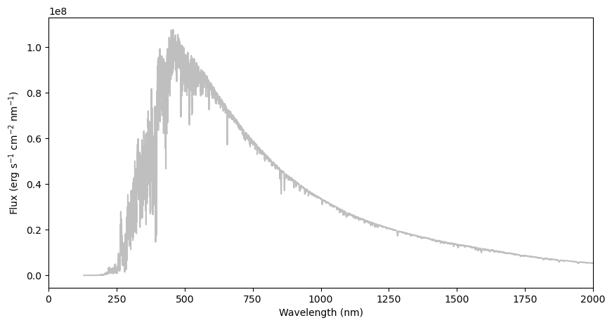
4. Let’s compare the grey flux with the real solar flux

In the plot below, I give you the solar spectrum, calculated with detailed stellar atmosphere models, that will emerge from the surface of the Sun. The wavelength axis is in \(\mathrm{nm}\), and the units of flux are \(\mathrm{erg}/\mathrm{s}/\mathrm{cm}^2/\mathrm{nm}\).

TODO: a. To the graph, add the curve from #3 that corresponds to the surface flux spectrum.

TODO b. When we made an approximation of a linear source function (e.g. when talked about Limb-darkening), we found that \(F_\lambda(\tau_\lambda=0) \sim \pi S_\lambda(\tau_\lambda=2/3)\). So in other words, if the source function is the Planck function, then the \(F_\lambda(\tau_\lambda=0)\) will be equal to the Plack function for a temperature that corresponds to the atmosphere layer that has an optical depth of 2/3, multiplied by \(\pi\).

i) Using our expression for the grey temperature structure (with \(q(\tau\sim2/3)\)) of the atmosphere, find \(T(\tau=2/3)\)

ii) Add a curve for the predicted observed \(F_\lambda\) in this approximation. There are many ways to do this:

• Computing the expression for \(B_\alpha\) from the worksheet and converting to \(B_\lambda\) with the code.

• Computing the expression for \(B_\nu\) from the worksheet and coverting to \(B_\lambda\) with the code.

• Analytically finding the expression for \(B_\lambda\) from the expression for \(B_\nu\) given in the worksheet.

Pick one and show your work and/or reasoning below (and don’t forget to multiply \(B\) by \(\pi\))

Enter your work and/or reasoning here:

fig, ax = plt.subplots(1,1, figsize=(10,5))
ax.set_xlim(0,2000)

ax.set_ylabel(r'Flux (erg s$^{-1}$ cm$^{-2}$ nm$^{-1}$)')
ax.set_xlabel('Wavelength (nm)')

# Loading a solar flux model from the MARCS stellar atmosphere models
file_url="https://raw.githubusercontent.com/veropetit/PHYS633-F2024/main/Book/L17-GreyAtmosphere/17-sun_wave.txt"
wave_sun = np.genfromtxt(file_url)
wave_sun = wave_sun/10*u.nm # Change the wavelength in nm

file_url="https://raw.githubusercontent.com/veropetit/PHYS633-F2024/main/Book/L17-GreyAtmosphere/17-sun_flux.txt"
flux_sun = np.genfromtxt(file_url)
flux_sun = flux_sun * u.erg/u.s/u.cm**2/u.nm * 10 # * 10 to go from /A to /nm.

ax.plot( wave_sun, convolve(flux_sun, Box1DKernel(31)), c="0.75" )

#--------------------------------

Teff = 5777*u.K # This is the effective temperature of the model

# I am giving your an array of wavelenght in nm to get you started.
wave = np.linspace(1,2000, 1000)*u.nm 

#--------------------------------

TODO: Please write a small paragraph with an interpretation of the result obtained:

Q: How good are the approximations?

Q: Which one does the best?

Q: Why does our model not showing any spectral lines?