02-GravityField (template)#
For reference: inserting images in Colab text files:#
There are two ways to insert images in markdown format in the text cells:
Quick direct markdown format:

or html codes which allows more formatting options
<img src="url" width="500">
If the image is hosted on GitHub:#
The link to the file on your GitHub will have this url (from the top bar):
https://github.com/veropetit/PHYS633-F2024/blob/main/Book/logo.png
But to embed it, you will need to add ?raw=true at the end of the url.
<img src="https://github.com/veropetit/PHYS633-F2024/blob/main/Book/logo.png?raw=true" width="500">
If the image is hosted on your Google Drive:#
First you will need to get a sharable link from Google Drive (make sure that the link is ‘viewable for everyone with the link’.
For example, here’s the sharable link to an image:
https://drive.google.com/file/d/1h7kgzG-uFEEg2RYr3iRnrRVV7zTDuf_L/view?usp=sharing
You will now need to change this link to embed the image. You need the image ID, which in this case is: 1h7kgzG-uFEEg2RYr3iRnrRVV7zTDuf_L
Then you can put this into a html image code like this:
<img src="https://drive.google.com/thumbnail?id=1h7kgzG-uFEEg2RYr3iRnrRVV7zTDuf_L&sz=s4000" width="100">
We start by importing the modules#
Numpy – operations on arrays and matrixes (and pi)
Matplotlib pyplot – plotting library
import numpy as np

import matplotlib.pyplot as plt
%matplotlib inline
# This option enables plots to be inline,
# as opposed to opening in a separate window.
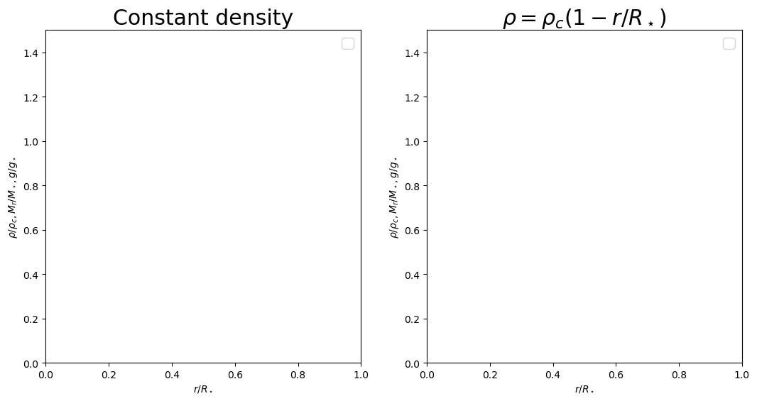
1. We will make a plot of the enclosed mass (\(M_r\)) and the gravitational acceleration (\(g\)) as a function of position inside the star (\(r\)).#
In class, we derived the “continuity equation”
In itself, we cannot yet solve for the structure of a star from this equation alone, because there are two quantities we do not know. As we will see in the next lecture, the fight between gravity and pressure (the “hydrostatic equilibrium”) will provide another equation that links the enclosed mass (through gravity) to the pressure.
But for now, the goal of this notebook is to
get a sense of how \(M_r\) and \(g(r)\) relates to the density.
get some practice in solving our differential equations of structure (like the continuity equation).
So in this notebook, we will pretend (for a moment) that we know how the density vary inside of a star and see what the resulting \(M_r(r)\) and \(g(r)\) would look like.
a. In class (left plot for constant density)#
Below I am showing you an example of a solution write-up for your notebook. As you can see, it is possible to type equations in latex, and include figure. In your write-up, I do not need (or want!) to see the purely algebra steps, and you can directly give the solution of unit-less integrals (after all, this is what Wolfram Alpha is for!)
We know from the continuity equation that \(dM_r=4\pi r^2 \rho(r) dr\). If we make a guess that the density is constant (\(rho(r) = \rho_0\)), we can find the mass enclosed mass by integrating the continuity equation on both sides. We will use the boundary condition that \(M_r=0\) when \(r=0\)
On the right side of the equation, I make a change of variable \(x=r/R_\star\) and pull all of the constant outside of the integral.
(This is what I mean by “I don’t need to see the purely algebra steps”):
TODO: finish writing up the solution for \(M_r(r)/M_\star\) and \(g(r)/g_\star\) for the constent density case
b. At home (right plot for linearly decreasing density)#
For our second plot, let imagine that the density varies like
where \(\rho_o\) is a constant.
TODO : Make the calculations below. Use Latex formatting to render the math (I give an example of what I am looking for in part a.)
Calculate and plot \(M_r/M_\star\), and \(g/g_\star\).
Calculate (you can do the numerical calculation in the code below) the value of \(\rho_o\) that our model implies if the star as a mass of \(1M_\odot\) and a radius of \(1R_\odot\)
Analytically find at which \(r/R_\star\) is \(g\) at its maximum, and add a vertical line at this position.
c. Code block for 1.a and 1.b#
TODO : Add a plot of \(M_r/M_\star\), and \(g/g_\star\) (that you calculated in part b.1 above), in the right-hand panel. Add a vertical line at the \(r/R_\star\) position at which \(g\) is at its maximum.
fig, ax = plt.subplots(1,2, figsize=(11,6))
# The subplot routine creates a figure object (in the variable "fig"), which contains
# and an array (here 2 plots) of plotting windows called "axes" (in the variable "ax")

plt.rcParams.update({'font.size': 18})
plt.rcParams.update({'font.family': 'Times New Roman'})
# Set the font and font size for the whole figure.

for item in ax:
    item.set_xlabel(r'$r/R_\star$') # the "r" is to say there is latex formatted strings.
    item.set_xlim(0,1)
    item.set_ylabel(r'$\rho/\rho_c, M_r/M_\star, g/g_\star$')
    item.set_ylim(0,1.5)
# ax is an vector of plot objects.
# we use a loop to set the title and limits of all plots to the same values

ax[0].set_title('Constant density')
ax[1].set_title(r'$\rho = \rho_c(1- r/R_\star)$')

#-----------------------------------------------------
#-----------------------------------------------------

#-----------------------------------------------------
# Part to do in class
#----

##################
# constant density
##################


####################
# Decreasing density at home
####################


#-----------------------------------------------------
# At home, add the curves for the g(s).
# Analytically find at which r/Rstar is g at its maximum, and add a vertical line at this position.
#----


#-----------------------------------------------------
#-----------------------------------------------------
#------------------------------------------------------
for item in ax:
    item.legend(loc=0, fontsize=15)
plt.tight_layout()
# arrange the plot nicely
No artists with labels found to put in legend.  Note that artists whose label start with an underscore are ignored when legend() is called with no argument.
No artists with labels found to put in legend.  Note that artists whose label start with an underscore are ignored when legend() is called with no argument.
TODO: Please write a small paragraph with an interpretation of the result obtained:
2. Learning reflection#
TODO: Please write a small reflection on what you have learned and why.
Suggestions: how does this notebook provide practice for the learning goal of this lecture? how does this topic fits within the learning goals of this course (could be science and/or techniques!), and how does it relates to other things that you have learned in other courses?