14-LimbDarkening (template)

We start by importing the modules

• Numpy – operations on arrays and matrixes (and pi)

• Matplotlib pyplot – plotting library

• Matplotlin patches – module that enables patches in plots

• Astropy units – defined quantities with units. We also import the CDS conversions

import numpy as np

import matplotlib.pyplot as plt
import matplotlib.patches as mpatches
%matplotlib inline 

from astropy import constants as const
import astropy.units as u
from astropy.units import cds
cds.enable()

<astropy.units.core._UnitContext at 0x10f21dd60>

1. In class: We can start by creating a polar grid (make sure to execute)

The grid represent the projected disk of a star on the sky, where \(\alpha\) is the distance from the center of the disk (let’s normalize the edge of the disk by \(\alpha=1\)), and \(\varphi\) is the azimutal angle aroung the center of the disk.

For later, we will also need the area on the sky represented by each grid point (\(\sim\alpha d\alpha d\varphi\)), as well as the value of \(u\). We saw earlier in the course (when discussing intensity vs flux) that we can relate the value of \(u\) and \(\alpha\) by

\[u = (1-\alpha^2)^{1/2}.\]

# Create a 2D grid in polar coordinates where 
# alpha is the radius from the center of the circle
# phi is the angle around the circle

n_phi = 10 # number of phi angles
n_alpha = 10   # number of radii

alpha = np.linspace(0, 1, n_alpha)
phi = np.radians(np.linspace(0, 360-(360/n_phi), n_phi))


#---------------------------------------
# In class


#alpha_grid = ....


#---------------------------------------
# We will need the projected area dA cos(theta)
# Area of a ring = 2 pi alpha dalpha
# Area of a rind segment = area of ring / number of segments

# Make sure to uncomment these after we have defined the grid

# area_grid = 2*np.pi * alpha_grid * (1.0/n_alpha) / n_phi

# and the value of u=cos(theta)

# u_grid = (1.0 - alpha_grid **2)**0.5

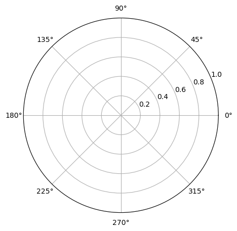
2. In class: Just a quick visualization of the grid

# We can get a figure in polar coordinate by using a "projection"
fig, ax = plt.subplots(1,1,subplot_kw=dict(projection='polar'), figsize=(5,5))

#------------------------------
# In class

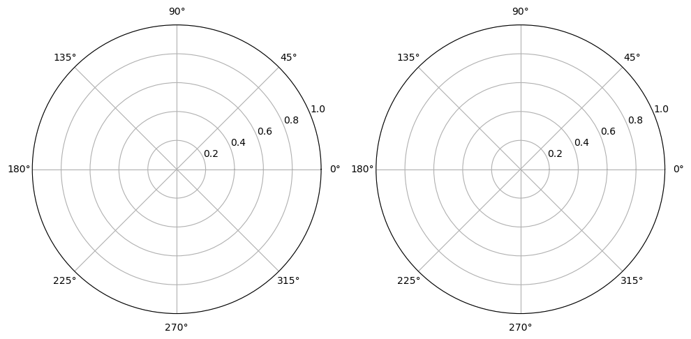
3. In class: let’s look at the effect of Limb-darkening

IMPORTANT Make sure to change the number of \(\alpha\) and \(\phi\) to 1000 in #1 and re-execute, to get a fine grid.

TODO: Below, provide an explanation (in words and math) that describes the calculations that we are performing in the code

fig, ax = plt.subplots(1,2,subplot_kw=dict(projection='polar'), figsize=(10,5))

# Loading a colormap
cmap = plt.cm.hot

#--------------------------------------------
# In class

Source_slope = 0.5


# Copy paste, change ax and source function slope



# ---------------------
plt.tight_layout()

TODO: Please write a small paragraph with an interpretation of the result obtained:

4. A simple estimate of planet transit

Each point in our polar grid can be transformed into cartesian coodinates, as

\[x = \alpha \cos(\varphi)\]

\[y = \alpha \sin(\varphi)\]

The cartesian equation for a circle if radius \(R\) centered on the coordinate \(x_o\) and \(y_o\) is

\[(x - x_o)^2 + (y - y_o)^2 = R^2.\]

Therefore, if we place a place a planet anywhere on our star’s disk, we can simply set the intensity to zero for every grid point where the following condition is met:

\[(x - x_o)^2 + (y - y_o)^2 \leq R^2!\]

To get the total flux coming out of the star, we can do a numerical integration by doing a sum of the product of \(I\) * Area on the disk. (You can convince yourself that this is correct from our discussion of the observed intensity vs observed flux.)

fig, ax = plt.subplots(subplot_kw=dict(projection='polar'), figsize=(5,5))


#--------------------------
# In class

Source_slope = 0.5

# 1. uncomment the itensity
#I = (1 + Source_slope*u_grid) / (1+Source_slope)


# 2. radius ratio of our planet


# 3. Take a copy of the intensity grid


# 4. Where is the planet?


#----------------------------------
# 5. uncomment the following to 
# make an image of the star + planet

#co = ax.pcolormesh(phi_grid, alpha_grid, I_transit, cmap=cmap, vmin=0)
#plt.colorbar(co)
#----------------------------------



# 6. Find the total flux coming out of the star without the planet


# 7. Find the total flux coming out of the star with the planet


#----------------------------------
# 8. Uncomment the following:

#print('The change is flux will be {:0.3g}'.format(Flux_transit / Flux_o))
#----------------------------------

5. At home: by using a series of \(x_o\) values, we can make a transit curve!

I provide a piece of code below that will create a transit curve, by making the planet (dark circle) cross the stellar disk horizontally.

If you study the code, you will see that there are different parameters that you can modify.

TODO: use the code below to make a study of how the shape of the planet transit changes according to the different parameters. Make sure to include the effect of different limb darkening in your study.

In the interpretation box below, you will describe the results of your study, using graphs that you will create with the code to support your results.

fig, ax = plt.subplots(1,1)


# Example for one set of parameters:
#-------------------------------------------------
#-------------------------------------------------
# Source_slope = 0.5
# I = (1 + Source_slope*u_grid) / (1+Source_slope)
# Flux_o = np.sum(I * area_grid)
# R = 0.1
# # Where is the planet?
# x0_array = np.linspace(-1-R,1+R,50) # array of xo to mimic a transit
# y0 = 0
# x_grid = alpha_grid * np.cos(phi_grid)
# y_grid = alpha_grid * np.sin(phi_grid)

# # The value of the transit are stored in "F_transit"
# F_transit = np.array([])    
# # Make the planet cross the star:
# for x0 in x0_array:
#   I_transit = np.copy(I)
#   planet = np.where( ( (x_grid - x0)**2 + (y_grid - y0)**2 ) <= R**2  )  
#   I_transit[planet] = 0.0
#   F_transit = np.append(F_transit, np.sum(I_transit * area_grid))

# ax.plot(x0_array, F_transit/Flux_o, c='k') 
#-------------------------------------------------
#-------------------------------------------------



# At home, make a few transit light curves for a set of parameters.
# How does the shape of the transit changes if 
# the radius of the planet, or the limb-darneking of the star changes?

TODO: Describe your results (and interpretation of your results) here.