ADM structure tutorial (using \(\tau\) Sco)

Step 1: create a potential field file

We first need to create a potential field file. In the Field Lines tutorial, we create a potential field object for a dipolar surface field.

In this example, let’s use the surface field map of \(\tau\) Sco from Donati+2006. The file tausco-br-donati.txt contains a longitude/latitude map of \(B_r\) at the surface. The ‘DONATI’ option in the Build_pot_field program reproduces this data by a series of spherical harmonics as the surface boundary condition for the potential field. The option l_max defines the cutoff for the harmomics (here, we choose to cut the surface harmonics at \(l=10\).

The input file ( looks like this:

&params
field_type_str = 'DONATI',
map_file = 'tausco-br-donati.txt',
l_max = 10,
pf_file = 'pf_tausco.h5'
/

And the command is:

$RICH/mag/field/build_pot_field < build_potential_donati.in

We should now have a pf_tausco.h5 file in our directory.

Step 2: calculate the ADM structure

Now, we can use this potential field object to construct a ADM volume structure using the Build_adm_vol program.

The input file (build_adm_vol.in here) is a bit longer for this one, and is structured into different categories – see the User’s manual for Build_adm_vol for all of the details.

&star
        M_star = 1.500000e+01       ! Stellar mass (M_sun)
        R_star = 5.200000e+00       ! Stellar radius (R_sun)
        T_eff  = 3.100000e+04       ! Stellar effective temperature (K)
/
&wind
        M_dot = 5.836637e-08        ! Mass-loss rate (M_sun/yr)
        v_inf = 2.000000e+03        ! Terminal velocity (km/s)
/
&adm
        delta = 0.1         ! Disk thickness (R_star)
        R_c = 64.           ! Closure radius (R_star)
/
&field
    ds = 1E-2           ! Segment length for field lines (R*)
    tol = 1E-3          ! Tolerance for field-line integrations (R*)
    R_source = 4.       ! Source-surface radius (R_star)
    R_outer = 64.       ! Outer extent of field lines (R_star)
/
&vol
    n_x = 128           ! x-dimension of adm_vol
    n_y = 128           ! y-dimension of adm_vol
    n_z = 128           ! z-dimension of adm_vol
    x_min = -5          ! x-minimum of adm_vol (R*)
    x_max = 5           ! x-maximum of adm_vol (R*)
    y_min = -5          ! y-minimum of adm_vol (R*)
    y_max = 5           ! y-maximum of adm_vol (R*)
    z_min = -5          ! z-maximum of adm_vol (R*)
    z_max = 5           ! z-maximum of adm_vol (R*)
    node_type = 'VERT'  ! Type of nodes (VERT or CELL)
/
&files
    pf_file = 'pf_tauscoL.h5'  ! Input pot_field file
    av_file = 'av_RS4.h5'  ! Output adm_vol file
/

A few notes:

• pf_file is the file containing the potential field we created in step 1.

• We here create a small grid (128x128x128) as a demonstration – this is a demanding calculation thus is may take some time on a laptop. The code is parrallelized however, and a high-res grid will run in a reasonble time on a multiprocessor machine (I suggest that you use a “screen” command still).

• Here, we set the R_source to 4 Rstar. Remember that the \(a_{lm}\) and \(b_{lm}\) defining the potential field solution are not stored in the potential field file – they are re-calculated on the fly each time a set_R_source command is issued. Thus you can use the same potential field file to make e.g. different ADM volumes files with various source radii.

• VERO NOTE TO SELF: check in my notes the diff between R_c and R_outer.

The command is:

$RICH/mag/adm/build_adm_vol < build_adm_vol.in

Using the python routine for a quick look

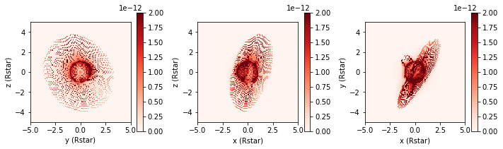
The plot_column_density function in the adm python module makes a graph of column density in 3 planes (xy, xz, and xy).

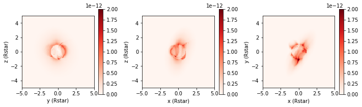
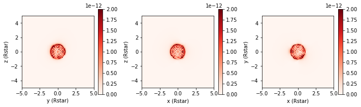
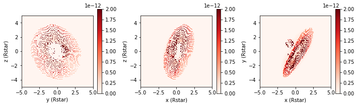
The keyword “type” selects which ADM region to utilize: * ‘cold’=downflow+upflow, * ‘hot’=shock region, * ‘upflow’, * ‘downflow’, * ‘all’

import matplotlib.pyplot as plt
import pyRich.magnetospheres as mag

adm = mag.load_adm_vol('av_RS4.h5')

fig, ax = adm.plot_column_density(type='all',cmap='Reds', vmax=0.2e-11)
plt.tight_layout()

fig, ax = adm.plot_column_density(type='downflow',cmap='Reds', vmax=0.2e-11)
plt.tight_layout()

fig, ax = adm.plot_column_density(type='upflow',cmap='Reds', vmax=0.2e-11)
plt.tight_layout()

fig, ax = adm.plot_column_density(type='hot',cmap='Reds', vmax=0.2e-11)
plt.tight_layout()